Visualising L1 and L2 Regularisation

Illustrating the fact L1 regularisation forces parameters to zero.

Introduction

You will often read that a big difference between L1 and L2 regularisation is that L1 regularisation forces parameters to zero, whereas L2 regularisation does not.

Michael Nielsen explains this via their effect on the update equations in gradient descent:

In both expressions the effect of regularization is to shrink the weights. This accords with our intuition that both kinds of regularization penalize large weights. But the way the weights shrink is different. In L1 regularization, the weights shrink by a constant amount toward 0. In L2 regularization, the weights shrink by an amount which is proportional to w. And so when a particular weight has a large magnitude, L1 regularization shrinks the weight much less than L2 regularization does. By contrast, when the magnitude is small, L1 regularization shrinks the weight much more than L2 regularization. The net result is that L1 regularization tends to concentrate the weight of the network in a relatively small number of high-importance connections, while the other weights are driven toward zero.

Alternatively, David Sotunbo provides a visualisation to explain the difference. This is great! However, one is left with the possibility that the particular cost function was cherry-picked to illustrate the desired effect.

Improving David’s visualisation

Building on top of David’s idea, I created visuals that illustrate what happens when you vary the cost function.

The framework

• We have a convex cost function C(x,y) = (x — a)^2 + (y — b)^2. This function’s contour plots are plotted in the visuals below.
• Without any restrictions, this cost function is minimised at x=a, y=b
• We see what happens if we restrict the values of the parameters x and y so that norm(x,y) < 1.norm will either be the L1 norm |x|+|y| or the L2 normsqrt(x^2 +y^2). This restriction is indicated as the blue shaded region in the visuals below.
• We vary a and b, and determine the parameters x and y that minimise C given the restriction on the norm. This is indicated by a red dot in the visuals below.

The visuals

Parameters restricted so that the L2-norm is less than 1

With the L2 restriction, we see the optimal parameter values change as we change the cost function.

Parameters restricted so that the L1-norm is less than 1

With the L1 restriction, the behaviour is strikingly different. Most of the time, the optimal parameters are at the corner of the region, where either x or y is equal to 0. In other words, L1-regularisation does indeed force parameters to zero!

Alternative visualisation

Though the visuals clearly illustrate the desired behaviour, the main issue is that they do not correspond exactly to L1 and L2 regularisation, in which the cost function is adjusted to include a regularisation term:

C(x,y) = (x — a)^2 + (y — b)^2 + lambda * R(x,y),

where R is either the L1 norm |x|+|y| or the (squared) L2 norm x^2 +y^2, and lambda is a hyper-parameter.

(Restricting the values of the parameters so thatnorm(x,y) < 1 does correspond to regularisation, but you have to define R appropriately. As a mini-exercise, try to determine thisR.)

Because the above visuals do not correspond exactly to L1 or L2 regularisation, I created an alternative visualisation.

The framework

• We have a cost function C(x,y) = (x — a)^2 + (y — b)^2 + lambda * R(x,y). I fixed lambda to be 1.
• For a givena and b, I determined the optimal parameters x' and y' of the resulting cost function.
• I vary a and b, producing many optimal parameters x' and y'. I plot all of these optimal parameters on a scatterplot.

The visuals

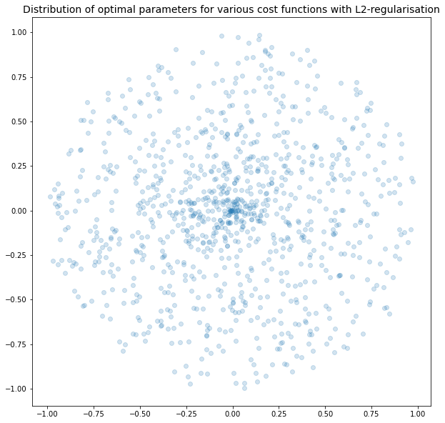
With L2 regularisation, we see that there is a preference for parameters to be closer to (0,0), but no preference for either parameter to be equal to 0.

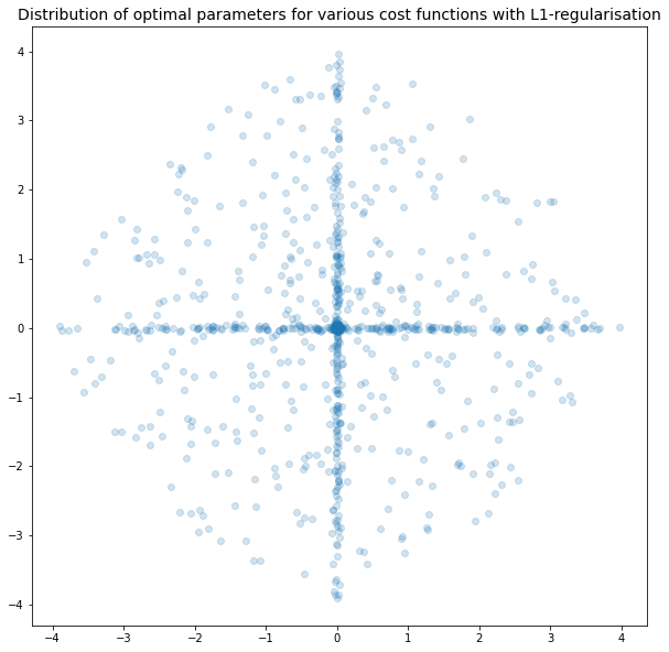
With L1 regularisation, we can clearly see that there is a preference for one of the parameters to be equal to 0. L1-regularisation does indeed force parameters to zero!

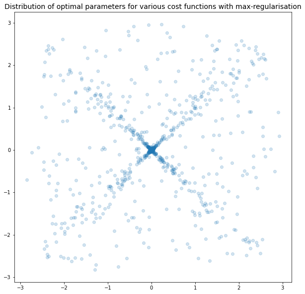
Max norm

To check your understanding of the four plots above, imagine how they would look if we replaced the L1 and L2 norms with the max norm, max_norm((x,y)) = max(|x|, |y|).

…

…

…

…

…

…

…

No really, take a couple of minutes to think this through if you already haven’t. You learn the most by actively engaging with the ideas rather than passively reading somebody else’s thoughts.

…

…

…

…

…

…

…

…

…

Here they are:

Conclusions

As with most aspects of data science, there are usually several ways of explaining an idea, and multiple layers of understanding available. I hope that these visuals have added to your understanding of regularisation.

Comments, suggestions, or thoughts are highly welcome! Please let me know what you think so I can improve for future posts. :)